Hey, guys in this article, I will tell teach you how to freeze rows and columns in excel.
If you usually work with large worksheets, it is very important that you familiarize yourself with the steps to freeze rows and columns in Excel. If you want Excel for Beginners Free.
Freeze rows and columns in Excel
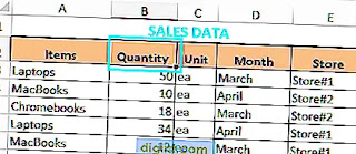
As you noticed, the column headings are no longer visible and are no longer visible when you scroll down an Excel worksheet.
Without the column headers visible, it becomes really difficult to enter new data in the correct columns or to view and compare the existing data.
An easy solution to this problem is to simply freeze the entire row of column headings. Once this is done, the column headings will be frozen and will always be visible when you scroll down.
Similarly, it is possible to freeze columns and freeze both rows and columns at the same time in Excel.
Note: Freezing rows or columns has no effect on printing, it only affects the way the worksheet appears on the screen.
Also read: How to Create a Pivot Table in Excel
1. Freeze rows in Excel
If you want to make the column headers stationary and always visible when you scroll down, you can follow the steps below to freeze the column header row.
1.1. Select the row (or the first cell in the row) immediately below the row containing the column headings.
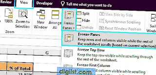
1.2. Then click on the View tab > click on Freeze Panels and then click on the Freeze Panels option from the drop-down menu.
This will freeze the column header row and this particular row will always remain visible when you scroll down the worksheet.
2. Freeze Columns in Excel
If the worksheet has multiple columns, you may want to make certain columns always visible when you scroll to the side of the worksheet (right or left).
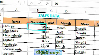
2.1. Select a cell immediately to the right of the column you want to freeze. In our case, we selected Cell B2 to freeze column A containing “Items”.
This will freeze column A and this particular column will always remain visible when you scroll sideways on the worksheet
3. Freeze both rows and columns in Excel
In some cases, you want to freeze the column header row and also freeze the first column or some selected columns in the worksheet.
To freeze both rows and columns, select the cell to the right of the column you want to freeze and below the row, you want to freeze.
In our case, we selected Cell B2 to freeze the second row of column headers and also freeze column A with "items".
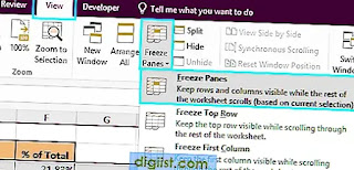
After selecting the right cell, from the drop-down menu, click View tab > Freeze Panels > Freeze Panels.
Now the rows above the selected cell remain frozen when you scroll down, and the columns to the left of the selected cell also remain frozen when you scroll to the side.
Unfreeze rows and columns panels in Excel
You can undo rows and columns in Excel at any time by clicking the View > Freeze Panes > Free Panes option from the drop-down menu.
The frozen rows or columns become free and no longer freeze or freeze when you scroll up or down.
Freeze Panes Not available in Excel
You may encounter an issue where the Pin Panels option is not available, grayed out, or not working. This problem is usually related to the worksheet that is in the "Page Layout" view. If you want How to Hide Columns in Excel.
To resolve this issue, click the View tab, and then click Normal or Page Break Preview.
The Freeze Panes option can also be disabled because the workbook is in protected mode.
However, this issue has been resolved in newer versions of Microsoft Excel and you will only encounter this issue while working on files created with an older version of Excel (older than Excel 2013).
I hope you understand how to freeze rows and columns in excel.
You may also visit here,


